Time Series Analysis and Understanding a Eurobond Fund with Prophet
<!–
–>
Want to share your content on R-bloggers? click here if you have a blog, or here if you don’t.
The Eurobonds are so popular in Turkey nowadays. The reason for this is that the CDS of Turkey fell for quite a while since the new economic outlook began, according to the economists. We will look into the factors that shape this trend in this article.
First, we build our data set with the components that we think are related to the Turkish Eurobonds.
library(tidyverse)
library(tidymodels)
library(timetk)
library(modeltime)
library(modelStudio)

#GPA(Eurobond Debt Instruments (FX) Fund of a private Turkish bank)
df_gpa <-
  read_csv("https://raw.githubusercontent.com/mesdi/blog/main/gpa.csv")

df_gpa_tidy %
  janitor::clean_names() %>%
  mutate(date = parse_date(date, "%m/%d/%Y")) %>%
  select(date, gpa = price)

#CDS(Turkey CDS 5 Years USD)
df_cds <-
  read_csv("https://raw.githubusercontent.com/mesdi/blog/main/cds.csv")

df_cds_tidy %
  janitor::clean_names() %>%
  mutate(date = parse_date(date, "%m/%d/%Y")) %>%
  select(date, cds = price)

#USDTRY(US Dollar Turkish Lira)
df_usdtry <-
  read_csv("https://raw.githubusercontent.com/mesdi/blog/main/usdtry.csv")

df_usdtry_tidy %
  janitor::clean_names() %>%
  mutate(date = parse_date(date, "%m/%d/%Y")) %>%
  select(date, usdtry = price)

#Federal Funds Effective Rate
df_fedfunds <-
  read_csv("https://raw.githubusercontent.com/mesdi/blog/main/fedfunds.csv")

##Converting Fed Funds data from monthly to weekly
library(padr)
df_fedfunds_tidy %
  janitor::clean_names() %>%
  thicken("week") %>%
  pad_by_time(date_week, .by = "week") %>%
  mutate(across(fedfunds, .fns = (x) ts_impute_vec(x, period = 1))) %>%
  select(date = date_week, fedfunds)

#Transforming the variables to PPP (Purchasing power parities)
#to see the changes(%) relative the last point
df_tidy %
  mutate(gpa = (gpa/first(gpa)*100) %>% round(2),
         cds = (cds/first(cds)*100) %>% round(2),
         usdtry = (usdtry/first(usdtry)*100) %>% round(2),
         fedfunds = (fedfunds/first(fedfunds)*100) %>% round(2))
Now that we have created our data set, we can examine the anomalies of the variables.
#Anomaly
df_all %>%
  pivot_longer(cols = -date, names_to = "vars") %>%
  plot_anomaly_diagnostics(date,
                           value,
                           .interactive = FALSE,
                           .facet_vars = vars,
                           .facet_ncol = 2)

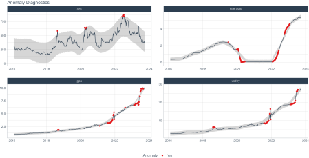
We can see that all variables but cds have had a lot of anomalies in the last few years. So we will choose the prophet model which is robust to outliers. Before moving on to our modeling, we will analyze the relations between all variables with the clustering method.
#Clustering
df_tsfeature %
  pivot_longer(cols = -date, names_to = "id") %>%
  group_by(id) %>%
  tk_tsfeatures(
    .date_var = date,
    .value    = value,
    .period   = 52,
    .features = c("frequency", "stl_features", "entropy", "acf_features", "mean"),
    .scale    = TRUE,
    .prefix   = "ts_"
  ) %>%
  ungroup()

set.seed(123)
tibble(
  cluster = df_tsfeature %>%
    select(-id) %>%
    as.matrix() %>%
    kmeans(centers = 3, nstart = 100) %>%
    pluck("cluster")
) %>%
  bind_cols(
    df_tsfeature
  ) %>%
  select(cluster, id) %>%
  right_join(df_all %>% pivot_longer(cols = -date, names_to = "id") ,
             by = "id") %>%
  group_by(id) %>%
  plot_time_series(
    date, value,
    .color_var   = cluster,
    .facet_ncol  = 2,
    .interactive = FALSE,
    .title = ""
  ) +
  theme(strip.text = ggtext::element_markdown(face = "bold"))

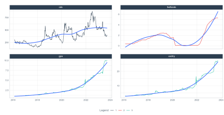
We can say that the gpa and usdtry variables are in the same cluster and look very similar. I wonder if we will see it in our model as well.
#Split into a train and test set
splits %
  timetk::time_series_split(assess = "1 year", cumulative = TRUE)

train <- training(splits)
test <- testing(splits)

#Modeling
df_rec <-
  recipe(gpa ~ ., data = train)


df_spec %
  set_engine(engine = "prophet")


set.seed(12345)
df_wflow_fit %
  add_recipe(df_rec) %>%
  add_model(df_spec) %>%
  fit(train)

#Calibration data
df_cal %
  modeltime_accuracy(metric_set = metric_set(rmse,rsq))

# A tibble: 1 × 5
#  .model_id .model_desc           .type  rmse   rsq
#
#1         1 PROPHET W/ REGRESSORS Test   2.40 0.989
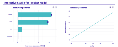
Based on the rsq and rmse values, our model looks very good. Now, we can calculate the variable importance values based on the model with the modeltStudio package. This will pop up the interactive dashboard on your browser, so you will be able to select variables on the right bottom for partial dependence.
#VIP(variable importance)
##Explainer object
library(DALEXtra)
explainer % select(-gpa),
    y     = train$gpa,
    label = "Prophet"
  )

##Model Studio
set.seed(1983)
modelStudio::modelStudio(explainer,
                         B = 100,
                         viewer = "browser")

Despite what economists say, the CDS(cds) seems to have little effect on the fund based on the dashboard. Besides, it looks like the most dominant effect is the USD/TRY(usdtry) rates’ and it has a strong linear relation to the GPA(gpa) fund. This confirms the inference we found earlier with clustering.
R-bloggers.com offers daily e-mail updates about R news and tutorials about learning R and many other topics. Click here if you’re looking to post or find an R/data-science job.
Want to share your content on R-bloggers? click here if you have a blog, or here if you don’t.
Continue reading: Time Series Analysis and Understanding a Eurobond Fund with Prophet