Leverage Effect

<!–

–>

The models we have been looking at do not differentiate between positive and negative residuals: both errors are treated the same. However, this does not align with reality, where the volatility resulting from a large negative return is higher than that for the corresponding positive return.

The reason for this is that a large negative return produces a significant reduction in market value. This, in turn, results in higher leverage. Why? Leverage is the ratio of debt to equity. Presumably a large negative return will not have an immediate impact on debt. But equity (assessed as the market value of all outstanding shares) will drop. Lower equity translates into higher leverage, making the company appear to be more reliant on debt.

Leverage Effect

To deal with the leverage asymmetry we need to have separate expressions for variance following positive and negative returns.

In a previous post we defined the model variance as

$$
sigma_t^2 = omega + alpha e_{t-1}^2 + beta sigma_{t-1}^2.
$$
This will still apply when the residual for the previous time step, (e_{t-1}), is positive. But for negative (e_{t-1}) the coefficient for the squared residual has a correction factor, (gamma):

$$
sigma_t^2 = omega + (alpha + gamma) e_{t-1}^2 + beta sigma_{t-1}^2.
$$
The coefficient of the squared residual is

• (alpha) when (e_{t-1} geq 0) and
• (alpha + gamma) when (e_{t-1} < 0).

This is the GJR (Glosten-Jagannathan-Runkle) GARCH model (original publication can be found here). The GJR GARCH model is based on the Standard GARCH model but also includes the leverage effect. When (gamma = 0) it reduces to the Standard GARCH model.

Standard GARCH Model

Start by modelling the ACC returns using a Standard GARCH ("sGARCH") model with a Normal Distribution.

specification <- ugarchspec(
  distribution.model = "norm",
  mean.model = list(armaOrder = c(0, 0)),
  variance.model = list(model = "sGARCH")
)

fit <- ugarchfit(data = ACC, spec = specification)

coef(fit)

          mu        omega       alpha1        beta1 
7.203541e-04 1.741503e-05 6.185551e-02 8.862047e-01 

The resulting model has fit the parameters (mu), (omega), (alpha) and (beta). The coefficient of the squared residuals in the volatility is 0.0619 for both positive and negative returns.

A news impact curve can be used to illustrate the symmetric response to negative and positive returns.

GJR GARCH Model

Now, using the same distribution but changing to a GJR GARCH ("gjrGARCH") model.

specification <- ugarchspec(
  distribution.model = "norm",
  mean.model = list(armaOrder = c(0, 0)),
  variance.model = list(model = "gjrGARCH")
)

fit <- ugarchfit(data = ACC, spec = specification)

coef(fit)

          mu        omega       alpha1        beta1       gamma1 
2.928785e-04 1.148255e-05 1.971500e-06 9.219841e-01 9.466123e-02 

This model also has a value for (gamma). The coefficient of the squared residuals is now 0.00000197 for positive residuals and 0.0947 for negative residuals. Negative returns clearly have a much larger impact on volatility!

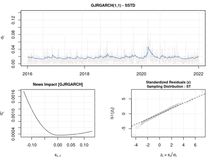
The news impact curve shows the asymmetry. Somewhat unrealistically this implies that positive returns have essentially no impact. That doesn’t seem quite right.

Given the asymmetry of the returns it would make more sense to use a skewed distribution, changing from "norm" to "sstd".

specification <- ugarchspec(
  distribution.model = "sstd",
  mean.model = list(armaOrder = c(0, 0)),
  variance.model = list(model = "gjrGARCH")
)

fit <- ugarchfit(data = ACC, spec = specification)

coef(fit)

          mu        omega       alpha1        beta1       gamma1         skew 
2.939585e-04 9.298925e-06 7.510285e-03 9.290941e-01 7.535600e-02 1.069799e+00 
       shape 
6.093299e+00 

Now positive returns do have an impact but it’s much smaller than that from negative returns.

Compare the volatility derived from the GJR GARCH model with a skewed distribution (blue) to that of the Standard GARCH model (red) with a Normal Distribution.

Midway through 2018 there’s a large positive return. This has an impact on the Standard GARCH model (red) but very little effect on the GJR GARCH model (blue). Looking at the return time series it’s apparent that there also really isn’t an appreciable increase in volatility at that time. However, in the first quarter of 2020 there’s a large negative return, which is accompanied by a significant escalation in volatility, which is reflected in both the Standard GARCH and GJR GARCH models.

Alternative Implementation

Let’s try with the {tsgarch} package.

library(tsgarch)

Create a GJR GARCH model specification with a Skewed Student-t Distribution.

specification <- garch_modelspec(
  ACC,
  model = "gjrgarch",
  distribution = "sstd",
  constant = TRUE
)

fit <- estimate(specification)

Now we have access to the statistical details of the estimated parameters. Not all of them are significant so we should probably think a bit harder about this model!

summary(fit)

GJRGARCH Model Summary

Coefficients:
             Estimate Std. Error t value Pr(>|t|)    
mu          2.916e-04  4.345e-04   0.671 0.502213    
omega       9.401e-06  3.615e-06   2.600 0.009316 ** 
alpha1      7.578e-03  9.968e-03   0.760 0.447142    
gamma1      7.571e-02  2.155e-02   3.513 0.000444 ***
beta1       9.286e-01  1.984e-02  46.809  < 2e-16 ***
skew        1.070e+00  3.928e-02  27.233  < 2e-16 ***
shape       6.100e+00  9.066e-01   6.729 1.71e-11 ***
persistence 9.750e-01  1.158e-02  84.230  < 2e-16 ***
---
Signif. codes:  0 '***' 0.001 '**' 0.01 '*' 0.05 '.' 0.1 ' ' 1

N: 1484
V(initial): 0.000339,  V(unconditional): 0.0003761
Persistence: 0.975
LogLik: 3952,  AIC:  -7888,  BIC: -7845.58

plot(fit)

Continue reading: Leverage Effect